Step-by-Step Guide — Building a Prediction Model in Python

Note from Towards Data Science’s editors: While we allow independent authors to publish articles in accordance with our rules and guidelines, we do not endorse each author’s contribution. You should not rely on an author’s works without seeking professional advice. See our Reader Terms for details.

Inthis post, I will show you how to build a program that can predict the price of a specific stock. This is a great project of using machine learning in finance. If we want a machine to make predictions for us, we should definitely train it well with some data. First, for those who are new to python, I will introduce it to you. Then, we will start working on our prediction model. As mentioned in the subtitle, we will be using Apple Stock Data. If you are wondering is it free to get that data, the answer is absolutely yes. The stock data is available on NASDAQ official website. The NASDAQ (National Association of Securities Dealers Automated Quotations) is an electronic stock exchange with more than 3,300 company listings.

The Apple stock data can be downloaded from here. On this website, you can also find stock data for different companies and practice your skills using different datasets. I can’t wait to see our prediction accuracy results, let’s get started!

Table of Contents:

• Python
• Libraries
• Understanding the Apple Stock Data
• Data Manipulation
• Data Visualization
• LSTM Prediction Model

Python

Python is a general-purpose programming language that is becoming ever more popular for analyzing data. Python also lets you work quickly and integrate systems more effectively. Companies from all around the world are utilizing Python to gather bits of knowledge from their data. 

Python for Finance — The Complete Beginner’s Guide

Simple and hands-on practice using Amazon Stock Data

Libraries

First things first, we have to install some libraries so that our program works. Here is a list of the libraries we will install: pandas, numpy, keras, and tensorflow. Tensorflow has to be installed so that keras can work.

Keras is an API designed for human beings, not machines. Keras follows best practices for reducing cognitive load: it offers consistent & simple APIs, it minimizes the number of user actions required for common use cases, and it provides clear & actionable error messages. It also has extensive documentation and developer guides.

We can install these libraries using Pip library manager:

pip install pandas numpy keras tensorflow

After the installation is completed, let’s import them into our code editor. Matplotlib is already included in Python that’s why we can import it without installing it.

import pandas as pd
import numpy as npimport matplotlib.pyplot as plt
%matplotlib inline
from matplotlib.pylab import rcParams
rcParams['figure.figsize']=20,10from keras.models import Sequential
from keras.layers import LSTM,Dropout,Densefrom sklearn.preprocessing import MinMaxScaler

Understanding the Apple Stock Data

Secondly, we will start loading the data into a dataframe, it is a good practice to take a look at it before we start manipulating it. This helps us to understand that we have the right data and to get some insights about it.

As mentioned earlier, for this exercise we will be using historical data of Apple. I thought Apple would be a good one to go with. After walking through with me on this project, you will learn some skills that will give you the ability to practice yourself using different datasets.

The dataframe that we will be using contains the closing prices of Apple stock of the last one year (Sept 16, 2019 — Sept 15, 2020).

Read Data

import pandas as pddf = pd.read_csv('aapl_stock_1yr.csv')

Head Method

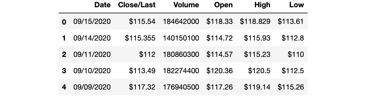
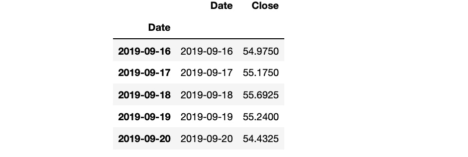
The first thing we’ll do to get some understanding of the data is using the head method. When you call the head method on the dataframe, it displays the first five rows of the dataframe. After running this method, we can also see that our data is sorted by the date index.

df.head()

Tail Method

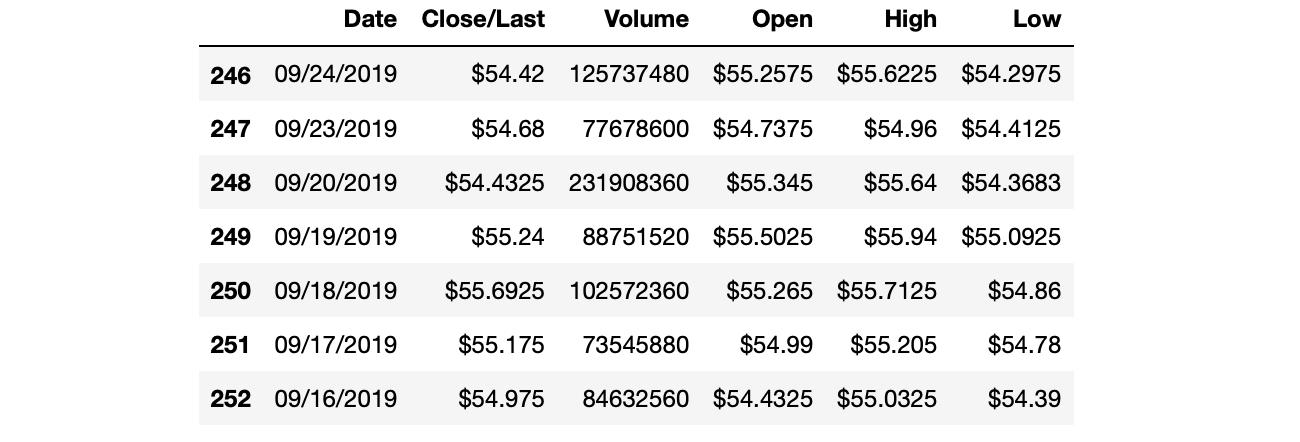
Another helpful method we will call is the tail method. It displays the last five rows of the dataframe. Let’s say if you want to see the last seven rows, you can input the value 7 as an integer between the parentheses.

df.tail(7)

Now we have an idea of the data. Let’s move to the next step which is data manipulation and making it ready for prediction.

Data Manipulation

Subsetting

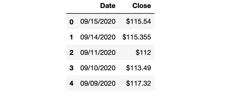
As you can see from the screenshots earlier, our dataframe has 6 columns. Do we need all of them? Of course not. For our prediction project, we will just need “Date” and “Close/Last” columns. Let’s get rid of the other columns then.

df = df[['Date', 'Close']]df.head()

Data Types

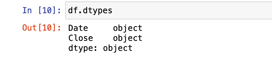
Now, let’s check the data types of the columns. Since we have a “$” sign in the closing price values, it might not be a float data type. When training the data, string datatype will not work with our model, so we have to convert it to float or integer type.

Before we convert it to float, let’s get rid of the “$” sign. Otherwise, conversion method will give us an error.

df = df.replace({'\$':''}, regex = True)

Great! Now, we can convert the “Closing price” data type to float. And we will also convert the “Date” data to datetime type.

df = df.astype({"Close": float})df["Date"] = pd.to_datetime(df.Date, format="%m/%d/%Y")df.dtypes

Index Column

This will be a short step. We will just define the dataframe’s index value as the date column. This will be helpful in the data visualization step.

df.index = df['Date']

Data Visualization

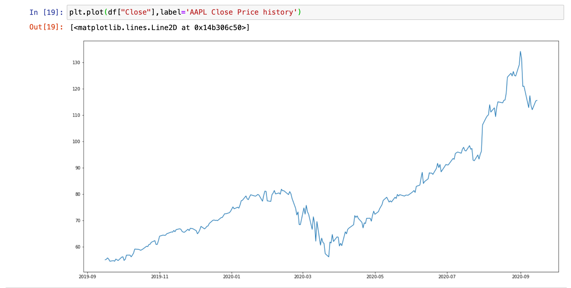
I will share a simple line chart with you just to give an idea of the stock price change in the last one year. We will also use the visualization method at the end to compare our prediction and reality.

plt.plot(df["Close"],label='Close Price history')

LSTM Prediction Model

In this step, we will do most of the programming. First, we need to do a couple of basic adjustments on the data. When our data is ready, we will use itto train our model. As a neural network model, we will use LSTM(Long Short-Term Memory) model. LSTM models work great when making predictions based on time-series datasets.

Data Preparation

df = df.sort_index(ascending=True,axis=0)data = pd.DataFrame(index=range(0,len(df)),columns=['Date','Close'])for i in range(0,len(data)):
    data["Date"][i]=df['Date'][i]
    data["Close"][i]=df["Close"][i]data.head()

Min-Max Scaler

scaler=MinMaxScaler(feature_range=(0,1))data.index=data.Date
data.drop(“Date”,axis=1,inplace=True)final_data = data.values
train_data=final_data[0:200,:]
valid_data=final_data[200:,:]scaler=MinMaxScaler(feature_range=(0,1))scaled_data=scaler.fit_transform(final_data)
x_train_data,y_train_data=[],[]
for i in range(60,len(train_data)):
    x_train_data.append(scaled_data[i-60:i,0])
    y_train_data.append(scaled_data[i,0])

LSTM Model

In this step, we are defining the Long Short-Term Memory model.

lstm_model=Sequential()
lstm_model.add(LSTM(units=50,return_sequences=True,input_shape=(x_train_data.shape[1],1)))
lstm_model.add(LSTM(units=50))
lstm_model.add(Dense(1))model_data=data[len(data)-len(valid_data)-60:].values
model_data=model_data.reshape(-1,1)
model_data=scaler.transform(model_data)

Train and Test Data

This step covers the preparation of the train data and the test data.

lstm_model.compile(loss=’mean_squared_error’,optimizer=’adam’)
lstm_model.fit(x_train_data,y_train_data,epochs=1,batch_size=1,verbose=2)X_test=[]
for i in range(60,model_data.shape[0]):
    X_test.append(model_data[i-60:i,0])
X_test=np.array(X_test)
X_test=np.reshape(X_test,(X_test.shape[0],X_test.shape[1],1))

Prediction Function

In this step, we are running the model using the test data we defined in the previous step.

predicted_stock_price=lstm_model.predict(X_test)
predicted_stock_price=scaler.inverse_transform(predicted_stock_price)

Prediction Result

Almost there, let’s check the accuracy of our model. We have around 250 rows, so I used 80% as train data and 20% as test data.

train_data=data[:200]
valid_data=data[200:]
valid_data['Predictions']=predicted_stock_price
plt.plot(train_data["Close"])
plt.plot(valid_data[['Close',"Predictions"]])

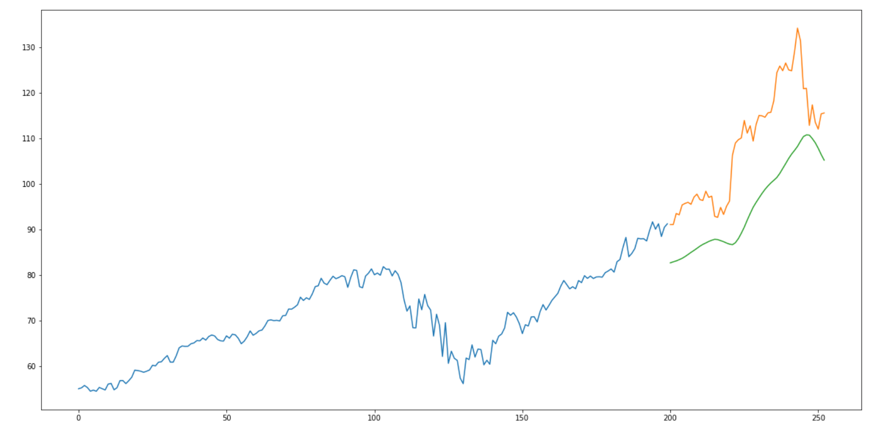
Congrats!! You have created a Python program that predicts the stock closing price of a company. Now, you have some idea of how to use machine learning in finance, you should try it with different stocks. Hoping that you enjoyed reading my article. Working on hands-on programming projects like this one is the best way to sharpen your coding skills.